ACCA F5考试:COST-VOLUME-PROFIT ANALYSIS (一)
1. THE OBJECTIVE OF CVP ANALYSIS
CVP analysis looks primarily at the effects of differing levels of activity on the financial results of a business. The reason for the particular focus on sales volume is because, in the short-run, sales price, and the cost of materials and labour, are usually known with a degree of accuracy. Sales volume, however, is not usually so predictable and therefore, in the short-run, profitability often hinges upon it.
2. Methods for calculating the break-even point
The break-even point is when total revenues and total costs are equal, that is, there is no profit but also no loss made. There are three methods for ascertaining this break-even point:
2.1 The equation method
Total revenue – total variable costs – total fixed costs = Profit
(USP x Q) – (UVC x Q) – FC = P (50Q) – (30Q) – 200,000 = P
Note: total fixed costs are used rather than unit fixed costs since unit fixed costs will vary depending on the level of output.
It would, therefore, be inappropriate to use a unit fixed cost since this would vary depending on output. Sales price and variable costs, on the other hand, are assumed to remain constant for all levels of output in the short-run, and, therefore, unit costs are appropriate.
2.2 The contribution margin method
This second approach uses a little bit of algebra to rewrite our equation above, concentrating on the use of the ‘contribution margin’. The contribution margin is equal to total revenue less total variable costs. Alternatively, the unit contribution margin (UCM) is the unit selling price (USP) less the unit variable cost (UVC). Hence, the formula from our mathematical method above is manipulated in the following way:
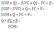
So, if P=0 (because we want to find the break-even point), then we would simply take our fixed costs and divide them by our unit contribution margin. We often see the unit contribution margin referred to as the ‘contribution per unit’.
Applying this approach to Company A again:
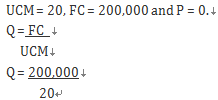
Therefore Q = 10,000 units
The contribution margin method uses a little bit of algebra to rewrite our equation above, concentrating on the use of the ‘contribution margin’.
2.3 The graphical method
With the graphical method, the total costs and total revenue lines are plotted on a graph; $ is shown on the y axis and units are shown on the x axis. The point where the total cost and revenue lines intersect is the break-even point. The amount of profit or loss at different output levels is represented by the distance between the total cost and total revenue lines. Figure 1 shows a typical break-even chart for Company A. The gap between the fixed costs and the total costs line represents variable costs.
Alternatively, a contribution graph could be drawn. While this is not specifically covered by the Paper F5 syllabus, it is still useful to see it. This is very similar to a break-even chart, the only difference being that instead of showing a fixed cost line, a variable cost line is shown instead.
Hence, it is the difference between the variable cost line and the total cost line that represents fixed costs.The advantage of this is that it emphasises contribution as it is represented by the gap between the total revenue and the variable cost lines. This is shown for Company A in Figure 2.
Finally, a profit–volume graph could be drawn, which emphasises the impact of volume changes on profit (Figure 3). This is key to the Paper F5 syllabus and is discussed in more detail later in this article.
3. When transfer prices are needed
3.1 Performance evaluation. The success of each division, whether measured by return on investment (ROI) or residual income (RI) will be changed. These measures might be interpreted as indicating that a division’s performance was unsatisfactory and could tempt management at head office to close it down.
3.2 Performance-related pay. If there is a system of performance-related pay, the remuneration of employees in each division will be affected as profits change. If they feel that their remuneration is affected unfairly, employees’ morale will be damaged.
3.3 Make/abandon/buy-in decisions. If the transfer price is very high, the receiving division might decide not to buy any components from the transferring division because it becomes impossible for it to make a positive contribution. That division might decide to abandon the product line or buy-in cheaper components from outside suppliers.
3.4 Motivation. Everyone likes to make a profit and this ambition certainly applies to the divisional managers. If a transfer price was such that one division found it impossible to make a profit, then the employees in that division would probably be demotivated. In contrast, the other division would have an easy ride as it would make profits easily, and it would not be motivated to work more efficiently.
3.5 Investment appraisal. New investment should typically be evaluated using a method such as net present value. However, the cash inflows arising from an investment are almost certainly going to be affected by the transfer price, so capital investment decisions can depend on the transfer price.
3.6 Taxation and profit remittance. If the divisions are in different countries, the profits earned in each country will depend on transfer prices. This could affect the overall tax burden of the group and could also affect the amount of profits that need to be remitted to head office.

精品好课免费试听